Model validation: Comparing a state estimate to observations
Contents
Model validation: Comparing a state estimate to observations#
We start by importing xarray, numpy and matplotlib as usual
import xarray as xr
import numpy as np
import matplotlib.pyplot as plt
%matplotlib inline
The model we will be using in this lecture is the Southen Ocean State Estimate (SOSE), which is available in the pangeo cloud as an intake catalogue. We will just follow the instructions how to load the data into our notebook and inspect the dataset.
import intake
cat = intake.Catalog("https://raw.githubusercontent.com/pangeo-data/pangeo-datastore/master/intake-catalogs/ocean.yaml")
ds_model = cat["SOSE"].to_dask()
ds_model
<xarray.Dataset>
Dimensions:   (XC: 2160, XG: 2160, YC: 320, YG: 320, Z: 42, Zl: 42, Zp1: 43, Zu: 42, time: 438)
Coordinates:
    Depth     (YC, XC) float32 dask.array<shape=(320, 2160), chunksize=(320, 2160)>
    PHrefC    (Z) float32 dask.array<shape=(42,), chunksize=(42,)>
    PHrefF    (Zp1) float32 dask.array<shape=(43,), chunksize=(43,)>
  * XC        (XC) float32 0.083333336 0.25 0.4166667 ... 359.75 359.9167
  * XG        (XG) float32 5.551115e-17 0.16666667 ... 359.6667 359.83334
  * YC        (YC) float32 -77.87497 -77.7083 -77.54163 ... -24.874966 -24.7083
  * YG        (YG) float32 -77.9583 -77.79163 -77.62497 ... -24.9583 -24.791632
  * Z         (Z) float32 -5.0 -15.5 -27.0 -39.5 ... -5075.0 -5325.0 -5575.0
  * Zl        (Zl) float32 0.0 -10.0 -21.0 -33.0 ... -4950.0 -5200.0 -5450.0
  * Zp1       (Zp1) float32 0.0 -10.0 -21.0 -33.0 ... -5200.0 -5450.0 -5700.0
  * Zu        (Zu) float32 -10.0 -21.0 -33.0 -46.0 ... -5200.0 -5450.0 -5700.0
    drC       (Zp1) float32 dask.array<shape=(43,), chunksize=(43,)>
    drF       (Z) float32 dask.array<shape=(42,), chunksize=(42,)>
    dxC       (YC, XG) float32 dask.array<shape=(320, 2160), chunksize=(320, 2160)>
    dxG       (YG, XC) float32 dask.array<shape=(320, 2160), chunksize=(320, 2160)>
    dyC       (YG, XC) float32 dask.array<shape=(320, 2160), chunksize=(320, 2160)>
    dyG       (YC, XG) float32 dask.array<shape=(320, 2160), chunksize=(320, 2160)>
    hFacC     (Z, YC, XC) float32 dask.array<shape=(42, 320, 2160), chunksize=(42, 320, 2160)>
    hFacS     (Z, YG, XC) float32 dask.array<shape=(42, 320, 2160), chunksize=(42, 320, 2160)>
    hFacW     (Z, YC, XG) float32 dask.array<shape=(42, 320, 2160), chunksize=(42, 320, 2160)>
    iter      (time) int64 dask.array<shape=(438,), chunksize=(438,)>
    rA        (YC, XC) float32 dask.array<shape=(320, 2160), chunksize=(320, 2160)>
    rAs       (YG, XC) float32 dask.array<shape=(320, 2160), chunksize=(320, 2160)>
    rAw       (YC, XG) float32 dask.array<shape=(320, 2160), chunksize=(320, 2160)>
    rAz       (YG, XG) float32 dask.array<shape=(320, 2160), chunksize=(320, 2160)>
  * time      (time) datetime64[ns] 2005-01-06 2005-01-11 ... 2010-12-31
Data variables:
    ADVr_SLT  (time, Zl, YC, XC) float32 dask.array<shape=(438, 42, 320, 2160), chunksize=(1, 42, 320, 2160)>
    ADVr_TH   (time, Zl, YC, XC) float32 dask.array<shape=(438, 42, 320, 2160), chunksize=(1, 42, 320, 2160)>
    ADVx_SLT  (time, Z, YC, XG) float32 dask.array<shape=(438, 42, 320, 2160), chunksize=(1, 42, 320, 2160)>
    ADVx_TH   (time, Z, YC, XG) float32 dask.array<shape=(438, 42, 320, 2160), chunksize=(1, 42, 320, 2160)>
    ADVy_SLT  (time, Z, YG, XC) float32 dask.array<shape=(438, 42, 320, 2160), chunksize=(1, 42, 320, 2160)>
    ADVy_TH   (time, Z, YG, XC) float32 dask.array<shape=(438, 42, 320, 2160), chunksize=(1, 42, 320, 2160)>
    DFrE_SLT  (time, Zl, YC, XC) float32 dask.array<shape=(438, 42, 320, 2160), chunksize=(1, 42, 320, 2160)>
    DFrE_TH   (time, Zl, YC, XC) float32 dask.array<shape=(438, 42, 320, 2160), chunksize=(1, 42, 320, 2160)>
    DFrI_SLT  (time, Zl, YC, XC) float32 dask.array<shape=(438, 42, 320, 2160), chunksize=(1, 42, 320, 2160)>
    DFrI_TH   (time, Zl, YC, XC) float32 dask.array<shape=(438, 42, 320, 2160), chunksize=(1, 42, 320, 2160)>
    DFxE_SLT  (time, Z, YC, XG) float32 dask.array<shape=(438, 42, 320, 2160), chunksize=(1, 42, 320, 2160)>
    DFxE_TH   (time, Z, YC, XG) float32 dask.array<shape=(438, 42, 320, 2160), chunksize=(1, 42, 320, 2160)>
    DFyE_SLT  (time, Z, YG, XC) float32 dask.array<shape=(438, 42, 320, 2160), chunksize=(1, 42, 320, 2160)>
    DFyE_TH   (time, Z, YG, XC) float32 dask.array<shape=(438, 42, 320, 2160), chunksize=(1, 42, 320, 2160)>
    DRHODR    (time, Zl, YC, XC) float32 dask.array<shape=(438, 42, 320, 2160), chunksize=(1, 42, 320, 2160)>
    ETAN      (time, YC, XC) float32 dask.array<shape=(438, 320, 2160), chunksize=(1, 320, 2160)>
    EXFswnet  (time, YC, XC) float32 dask.array<shape=(438, 320, 2160), chunksize=(1, 320, 2160)>
    KPPg_SLT  (time, Zl, YC, XC) float32 dask.array<shape=(438, 42, 320, 2160), chunksize=(1, 42, 320, 2160)>
    KPPg_TH   (time, Zl, YC, XC) float32 dask.array<shape=(438, 42, 320, 2160), chunksize=(1, 42, 320, 2160)>
    PHIHYD    (time, Z, YC, XC) float32 dask.array<shape=(438, 42, 320, 2160), chunksize=(1, 42, 320, 2160)>
    SALT      (time, Z, YC, XC) float32 dask.array<shape=(438, 42, 320, 2160), chunksize=(1, 42, 320, 2160)>
    SFLUX     (time, YC, XC) float32 dask.array<shape=(438, 320, 2160), chunksize=(1, 320, 2160)>
    SIarea    (time, YC, XC) float32 dask.array<shape=(438, 320, 2160), chunksize=(1, 320, 2160)>
    SIatmFW   (time, YC, XC) float32 dask.array<shape=(438, 320, 2160), chunksize=(1, 320, 2160)>
    SIatmQnt  (time, YC, XC) float32 dask.array<shape=(438, 320, 2160), chunksize=(1, 320, 2160)>
    SIdHbATC  (time, YC, XC) float32 dask.array<shape=(438, 320, 2160), chunksize=(1, 320, 2160)>
    SIdHbATO  (time, YC, XC) float32 dask.array<shape=(438, 320, 2160), chunksize=(1, 320, 2160)>
    SIdHbOCN  (time, YC, XC) float32 dask.array<shape=(438, 320, 2160), chunksize=(1, 320, 2160)>
    SIdSbATC  (time, YC, XC) float32 dask.array<shape=(438, 320, 2160), chunksize=(1, 320, 2160)>
    SIdSbOCN  (time, YC, XC) float32 dask.array<shape=(438, 320, 2160), chunksize=(1, 320, 2160)>
    SIempmr   (time, YC, XC) float32 dask.array<shape=(438, 320, 2160), chunksize=(1, 320, 2160)>
    SIfu      (time, YC, XG) float32 dask.array<shape=(438, 320, 2160), chunksize=(1, 320, 2160)>
    SIfv      (time, YG, XC) float32 dask.array<shape=(438, 320, 2160), chunksize=(1, 320, 2160)>
    SIheff    (time, YC, XC) float32 dask.array<shape=(438, 320, 2160), chunksize=(1, 320, 2160)>
    SIhsnow   (time, YC, XC) float32 dask.array<shape=(438, 320, 2160), chunksize=(1, 320, 2160)>
    SIsnPrcp  (time, YC, XC) float32 dask.array<shape=(438, 320, 2160), chunksize=(1, 320, 2160)>
    SItflux   (time, YC, XC) float32 dask.array<shape=(438, 320, 2160), chunksize=(1, 320, 2160)>
    SIuheff   (time, YC, XG) float32 dask.array<shape=(438, 320, 2160), chunksize=(1, 320, 2160)>
    SIuice    (time, YC, XG) float32 dask.array<shape=(438, 320, 2160), chunksize=(1, 320, 2160)>
    SIvheff   (time, YG, XC) float32 dask.array<shape=(438, 320, 2160), chunksize=(1, 320, 2160)>
    SIvice    (time, YG, XC) float32 dask.array<shape=(438, 320, 2160), chunksize=(1, 320, 2160)>
    TFLUX     (time, YC, XC) float32 dask.array<shape=(438, 320, 2160), chunksize=(1, 320, 2160)>
    THETA     (time, Z, YC, XC) float32 dask.array<shape=(438, 42, 320, 2160), chunksize=(1, 42, 320, 2160)>
    TOTSTEND  (time, Z, YC, XC) float32 dask.array<shape=(438, 42, 320, 2160), chunksize=(1, 42, 320, 2160)>
    TOTTTEND  (time, Z, YC, XC) float32 dask.array<shape=(438, 42, 320, 2160), chunksize=(1, 42, 320, 2160)>
    UVEL      (time, Z, YC, XG) float32 dask.array<shape=(438, 42, 320, 2160), chunksize=(1, 42, 320, 2160)>
    VVEL      (time, Z, YG, XC) float32 dask.array<shape=(438, 42, 320, 2160), chunksize=(1, 42, 320, 2160)>
    WSLTMASS  (time, Zl, YC, XC) float32 dask.array<shape=(438, 42, 320, 2160), chunksize=(1, 42, 320, 2160)>
    WTHMASS   (time, Zl, YC, XC) float32 dask.array<shape=(438, 42, 320, 2160), chunksize=(1, 42, 320, 2160)>
    WVEL      (time, Zl, YC, XC) float32 dask.array<shape=(438, 42, 320, 2160), chunksize=(1, 42, 320, 2160)>
    oceFreez  (time, YC, XC) float32 dask.array<shape=(438, 320, 2160), chunksize=(1, 320, 2160)>
    oceQsw    (time, YC, XC) float32 dask.array<shape=(438, 320, 2160), chunksize=(1, 320, 2160)>
    oceTAUX   (time, YC, XG) float32 dask.array<shape=(438, 320, 2160), chunksize=(1, 320, 2160)>
    oceTAUY   (time, YG, XC) float32 dask.array<shape=(438, 320, 2160), chunksize=(1, 320, 2160)>
    surForcS  (time, YC, XC) float32 dask.array<shape=(438, 320, 2160), chunksize=(1, 320, 2160)>
    surForcT  (time, YC, XC) float32 dask.array<shape=(438, 320, 2160), chunksize=(1, 320, 2160)>
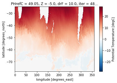
This dataset has a lot of output variables. For this lecture we are going to focus on sea surface temperature. In the model this is represented by the surfac layer in the vertical (dimension Z) of the temperature dataarray THETA.
Lets create a new sst_model dataarray and plot the first time step.
sst_model = ds_model.THETA.isel(Z=0)
sst_model.isel(time=0).plot()
<matplotlib.collections.QuadMesh at 0x7f466c068710>
As the name suggests, this model output is not global, but instead focusses on the Southern Ocean. A common analysis step is model validation - comparing model output to an observation of the same variable. We will use the previously used sea surface temperature dataset.
We load the dataset as before, but limit the latitude dimension to exclude values in the tropics and the northern hemisphere.
Note that the
londimension in the dataset is given in descending order, e.g. the first value is the northernmost. You can change the order by applyingsortby('lat'), which will reshuffle the full dataset so thatlatvalues are monotonically increasing.
# xr.set_options(display_style='html') # !!! need to update xarray for this?
url = 'http://www.esrl.noaa.gov/psd/thredds/dodsC/Datasets/noaa.ersst.v5/sst.mnmean.nc'
ds_obs = xr.open_dataset(url).chunk({'time': 12}).sortby('lat')
# restrict the obs to the southern ocean
ds_obs = ds_obs.sel(lat=slice(-90, -25))
ds_obs
<xarray.Dataset>
Dimensions:    (lat: 32, lon: 180, nbnds: 2, time: 1990)
Coordinates:
  * lat        (lat) float64 -88.0 -86.0 -84.0 -82.0 ... -32.0 -30.0 -28.0 -26.0
  * lon        (lon) float64 0.0 2.0 4.0 6.0 8.0 ... 352.0 354.0 356.0 358.0
  * time       (time) datetime64[ns] 1854-01-01 1854-02-01 ... 2019-10-01
Dimensions without coordinates: nbnds
Data variables:
    time_bnds  (time, nbnds) float64 dask.array<shape=(1990, 2), chunksize=(12, 2)>
    sst        (time, lat, lon) float32 dask.array<shape=(1990, 32, 180), chunksize=(12, 32, 180)>
Attributes:
    climatology:                     Climatology is based on 1971-2000 SST, X...
    description:                     In situ data: ICOADS2.5 before 2007 and ...
    keywords_vocabulary:             NASA Global Change Master Directory (GCM...
    keywords:                        Earth Science > Oceans > Ocean Temperatu...
    instrument:                      Conventional thermometers
    source_comment:                  SSTs were observed by conventional therm...
    geospatial_lon_min:              -1.0
    geospatial_lon_max:              359.0
    geospatial_laty_max:             89.0
    geospatial_laty_min:             -89.0
    geospatial_lat_max:              89.0
    geospatial_lat_min:              -89.0
    geospatial_lat_units:            degrees_north
    geospatial_lon_units:            degrees_east
    cdm_data_type:                   Grid
    project:                         NOAA Extended Reconstructed Sea Surface ...
    original_publisher_url:          http://www.ncdc.noaa.gov
    References:                      https://www.ncdc.noaa.gov/data-access/ma...
    source:                          In situ data: ICOADS R3.0 before 2015, N...
    title:                           NOAA ERSSTv5 (in situ only)
    history:                         created 07/2017 by PSD data using NCEI's...
    institution:                     This version written at NOAA/ESRL PSD: o...
    citation:                        Huang et al, 2017: Extended Reconstructe...
    platform:                        Ship and Buoy SSTs from ICOADS R3.0 and ...
    standard_name_vocabulary:        CF Standard Name Table (v40, 25 January ...
    processing_level:                NOAA Level 4
    Conventions:                     CF-1.6, ACDD-1.3
    metadata_link:                   :metadata_link = https://doi.org/10.7289...
    creator_name:                    Boyin Huang (original)
    date_created:                    2017-06-30T12:18:00Z (original)
    product_version:                 Version 5
    creator_url_original:            https://www.ncei.noaa.gov
    license:                         No constraints on data access or use
    comment:                         SSTs were observed by conventional therm...
    summary:                         ERSST.v5 is developed based on v4 after ...
    dataset_title:                   NOAA Extended Reconstructed SST V5
    data_modified:                   2019-11-04
    DODS_EXTRA.Unlimited_Dimension:  time
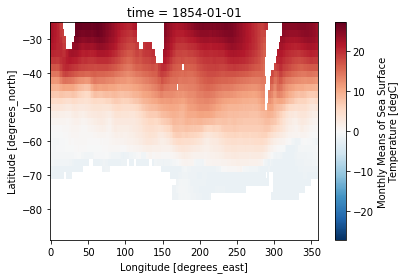
Lets now define a new dataarray so that we have a consistent naming between the model output and observations. As before we also plot the first time step of the data.
sst_obs = ds_obs.sst
sst_obs.isel(time=0).plot()
<matplotlib.collections.QuadMesh at 0x7f465431c8d0>
Considerations for model validation#
Now that we have both datasets loaded, how do we approach the model validation?
It is always crucial to put some thought into which time periods of a model and observations are actually comparable. In this case both should be directly comparable since SOSE is a state estimate, which incorporates observations to estimate the state of the ocean at the time observations were taken (and in between). If however the model data would be from a fully coupled climate model, we would have to take e.g. long averages due to the fact that internal variability - like for instance ENSO - can not be expected to happen in the same year as observations. But since we chose a state estimate, we can actually compare the data in a single year or even month (this will save us some computing time, but if you are interested, go ahead and choose a longer averaging period below and compare the results).
Now select a time period that overlaps between model and observations, e.g. the year 2009 and average over the year.
sst_model = sst_model.sel(time='2009').mean('time').load()
sst_obs = sst_obs.sel(time='2009').mean('time').load()
/srv/conda/envs/notebook/lib/python3.7/site-packages/dask/array/numpy_compat.py:38: RuntimeWarning: invalid value encountered in true_divide
  x = np.divide(x1, x2, out)
For later we will also rename the model dimensions XC and YC into lon and lat, so that both model and observations are named consistently.
sst_model = sst_model.rename({'XC':'lon', 'YC':'lat'})
We can now plot both fields next to each other. By specifying vmax=30 in the plot command, we ensure that both plots have the exact same colorbar.
plt.figure(figsize=[16,4])
plt.subplot(1,2,1) # !!! is this taught before?
sst_obs.plot(vmax=30) # make sure to have the same colorlimit
plt.ylim(-80, -24)

plt.subplot(1,2,2)
sst_model.plot(vmax=30)
<matplotlib.collections.QuadMesh at 0x7f4654183c50>
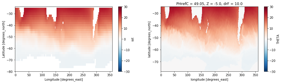
This looks nice and the large scale structure (colder waters near Antarctica) agree. But since temperature differs over such a wide range, it is hard to quantify the differences with the naked eye. Naturally we would want to plot the difference between both datasets.
Regridding via interpolation#
There is however a major problem: Both datasets are on a different grid - the model has a much higher resolution (~ 1/5 deg) than the observations (~ 2 degree). In the model we can see signs of mesoscale eddies, even in the yearly average.
To compare the dataset directly they have to be on the same grid, e.g. each point of the array has to correspond to the same position.
We have 3 options to achieve this:
Regrid the lower resolution dataset (observations) onto the higher resolution dataset (model).
Regrid the higher resolution dataset (model) onto the lower resolution dataset (observations).
Define a completely new grid and regrid both datasets onto that.
Both 1. and 2. have unique advantages and disadvantages, whereas 3. can share some or all of these, depending on whether the new grid is defined on a higher, lower or intermediate resolution compared to the two datasets.
Lets try both approaches and see how they compare. For this step we will use xesmf a very powerful geospatial regridding tool.
import xesmf as xe
To regrid a dataarray with xesmf you need to execute the following steps:
Create a target grid dataset (this can also be an existing dataset)
Note: Rename the dataset appropriately. xesmf expects longitude and latitude to be labelled as
lonandlat(this is the reason we renamed the model dataset previously).Create a
regridderobject (using the target grid and the source dataset - e.g. the dataset that should be regridded)Note: You might have to clean existing files that the regridder might have written out using
regridder.clean_weight_file()(this is only needed if the regridder has been previously applied, but it does not hurt to apply it just in case)Apply the
regridderto a dataset, e.g.regridder(ds)
We will start by regridding the low resolution observations onto the high resolution model grid, by using linear interpolation in two dimensions (bilinear) and specifying that our domain is periodic.
regridder = xe.Regridder(sst_obs, sst_model, 'bilinear', periodic=True) #since this is global we need to pass periodic
regridder.clean_weight_file()
regridder
Create weight file: bilinear_32x180_320x2160_peri.nc
Remove file bilinear_32x180_320x2160_peri.nc
xESMF Regridder
Regridding algorithm:       bilinear
Weight filename:            bilinear_32x180_320x2160_peri.nc
Reuse pre-computed weights? False
Input grid shape:           (32, 180)
Output grid shape:          (320, 2160)
Output grid dimension name: ('lat', 'lon')
Periodic in longitude?      True
We can now apply the regridder to the observed sea surface temperature.
sst_obs_regridded = regridder(sst_obs)
sst_obs_regridded
<xarray.DataArray 'sst' (lat: 320, lon: 2160)>
array([[nan, nan, nan, ..., nan, nan, nan],
       [nan, nan, nan, ..., nan, nan, nan],
       [nan, nan, nan, ..., nan, nan, nan],
       ...,
       [ 0.,  0.,  0., ...,  0.,  0.,  0.],
       [ 0.,  0.,  0., ...,  0.,  0.,  0.],
       [ 0.,  0.,  0., ...,  0.,  0.,  0.]])
Coordinates:
  * lon      (lon) float32 0.083333336 0.25 0.4166667 ... 359.75 359.9167
  * lat      (lat) float32 -77.87497 -77.7083 -77.54163 ... -24.874966 -24.7083
Attributes:
    regrid_method:  bilinear
You see that the size of the dimensions has increased. It is now the same as the model data. Lets see how the regridded data compares.
plt.figure(figsize=[16,4])
plt.subplot(1,2,1)
sst_obs_regridded.plot(vmax=30) # make sure to have the same colorlimit
# plt.ylim(-80, -24)

plt.subplot(1,2,2)
sst_model.plot(vmax=30)
<matplotlib.collections.QuadMesh at 0x7f4648031320>
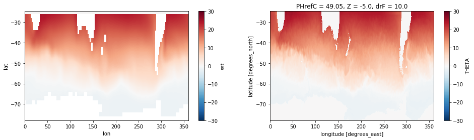
The observations now have more datapoints and look a lot smoother, but since the values are just linearly interpolated, there is no new information on smaller scales.
Now lets compare both estimates by computing the difference.
diff = sst_model - sst_obs_regridded
diff.plot(vmax=2)
<matplotlib.collections.QuadMesh at 0x7f4643f08320>
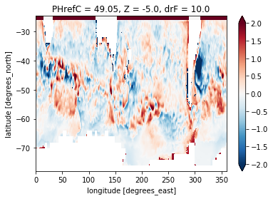
We can see that the model sea surface temperature is quite a bit different (up to 2 deg C in some places). But the comparison is hindered by a lot of smaller scale structure that stems from eddies in the model data, which are not resolved in the observations.
This is the major disadvantage of Method 1. from above: The comparison becomes ‘unfair’ because we are usually only interested on larger scale differences. Even if the observations would have a higher resolution, from our physical understanding we would not expect that turbulent features like ocean eddies would happen at the exact same space and time in the model as the observations.
So how do we solve this issue? Lets look at method 2. to compare the model and observations on a lower resolution. We first try the exact same procedure as befor (linear interpolation), but switch the source and target datasets.
regridder = xe.Regridder(sst_model,sst_obs, 'bilinear', periodic=True) #since this is global we need to pass periodic
regridder.clean_weight_file()
sst_model_regridded = regridder(sst_model)
sst_model_regridded
Create weight file: bilinear_320x2160_32x180_peri.nc
Remove file bilinear_320x2160_32x180_peri.nc
<xarray.DataArray 'THETA' (lat: 32, lon: 180)>
array([[ 0.      ,  0.      ,  0.      , ...,  0.      ,  0.      ,  0.      ],
       [ 0.      ,  0.      ,  0.      , ...,  0.      ,  0.      ,  0.      ],
       [ 0.      ,  0.      ,  0.      , ...,  0.      ,  0.      ,  0.      ],
       ...,
       [20.185935, 19.964374, 19.690668, ..., 20.646542, 20.335984, 20.317114],
       [20.801154, 20.477957, 20.144566, ..., 21.67011 , 21.22205 , 21.067159],
       [20.903206, 20.605169, 20.364102, ..., 21.828444, 21.537927, 21.231561]])
Coordinates:
    PHrefC   float32 49.05
    Z        float32 -5.0
    drF      float32 10.0
  * lon      (lon) float64 0.0 2.0 4.0 6.0 8.0 ... 350.0 352.0 354.0 356.0 358.0
  * lat      (lat) float64 -88.0 -86.0 -84.0 -82.0 ... -32.0 -30.0 -28.0 -26.0
Attributes:
    regrid_method:  bilinear
Lets compare the original observations against the regridded model data as before
diff = sst_model_regridded - sst_obs
diff.plot(vmax=2)
<matplotlib.collections.QuadMesh at 0x7f4643ebf4a8>
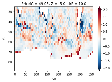
That was easy enough, but there is a problem with this approach. Using linear interpolation works very well when we ‘upsample’ (going from lower to higher resolution), since most of the interpolated points are between the wider spaced original data. If we ‘downsample’ (going from higher resolution to lower resolution), this method will only use the two nearest points to infer a new value. This means most of the high resolution source data is not taken into consideration, and small noisy features can have a disproportionate influence on the regridded data. It also implies that properties like tracer concentrations over the full domain are not necessarily conserved.
We can plot the original and the downsampled modeldata along a constant latitude to illustrate the problem
sample_lat = -46
sst_model.sel(lat=sample_lat, method='nearest').sel(lon=slice(0,40)).plot(marker='*')
sst_model_regridded.sel(lat=sample_lat, method='nearest').sel(lon=slice(0,40)).plot(marker='*')
[<matplotlib.lines.Line2D at 0x7f4638207898>]
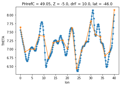
As you can see the upsampled datapoints depend highly on the position of the target grid. What we should rather do in this case is average values around the wider target grid. This can be achieved by using a different method in xesmf.
Regridding using conservative interpolation#
The conservative option will take an average over several grid cells to reduce the resolution of the model. This ensures that no information is discarded and that for instance adjacent positive and negative anomalies are not increasing the noise in the regridded data.
This method is always preferable, when moving to lower resolutions, especially when the data is not very smooth. Unfortunately this also requires some more input parameter, namely the bounding coordinates of each gridpoint (in addition to the center or tracer coordinate; see schematic in the introduction). xesmf expects those coordinates to be named lon_b and lat_b.
When we look carefully at the model data, these bounding coordinates are already given (as the coodinates for the \(u\) and \(v\) velocities on a staggered grid - XC and YC respectively), but xesmf requires a bounding value at each side (This model does only provides the same amount of coordinate values for both tracer and velocity points).
We have two options: a) Remove one of the tracer points and leave the velocity points as is, or b) add an additional coordinate value.
Since the model has a significantly higher resolution, we will chose the simpler way a) and just remove one tracer point, omitting one out of 10 points for the new coarse grid (which is acceptable in this case).
modified_grid_model = ds_model.isel(XC=slice(0,-1),
                                    YC=slice(0,-1)).rename({'XC':'lon',
                                                            'XG':'lon_b',
                                                            'YC':'lat',
                                                            'YG':'lat_b'})

modified_grid_model
<xarray.Dataset>
Dimensions:   (Z: 42, Zl: 42, Zp1: 43, Zu: 42, lat: 319, lat_b: 320, lon: 2159, lon_b: 2160, time: 438)
Coordinates:
    Depth     (lat, lon) float32 dask.array<shape=(319, 2159), chunksize=(319, 2159)>
    PHrefC    (Z) float32 dask.array<shape=(42,), chunksize=(42,)>
    PHrefF    (Zp1) float32 dask.array<shape=(43,), chunksize=(43,)>
  * lon       (lon) float32 0.083333336 0.25 0.4166667 ... 359.58334 359.75
  * lon_b     (lon_b) float32 5.551115e-17 0.16666667 ... 359.6667 359.83334
  * lat       (lat) float32 -77.87497 -77.7083 ... -25.041632 -24.874966
  * lat_b     (lat_b) float32 -77.9583 -77.79163 ... -24.9583 -24.791632
  * Z         (Z) float32 -5.0 -15.5 -27.0 -39.5 ... -5075.0 -5325.0 -5575.0
  * Zl        (Zl) float32 0.0 -10.0 -21.0 -33.0 ... -4950.0 -5200.0 -5450.0
  * Zp1       (Zp1) float32 0.0 -10.0 -21.0 -33.0 ... -5200.0 -5450.0 -5700.0
  * Zu        (Zu) float32 -10.0 -21.0 -33.0 -46.0 ... -5200.0 -5450.0 -5700.0
    drC       (Zp1) float32 dask.array<shape=(43,), chunksize=(43,)>
    drF       (Z) float32 dask.array<shape=(42,), chunksize=(42,)>
    dxC       (lat, lon_b) float32 dask.array<shape=(319, 2160), chunksize=(319, 2160)>
    dxG       (lat_b, lon) float32 dask.array<shape=(320, 2159), chunksize=(320, 2159)>
    dyC       (lat_b, lon) float32 dask.array<shape=(320, 2159), chunksize=(320, 2159)>
    dyG       (lat, lon_b) float32 dask.array<shape=(319, 2160), chunksize=(319, 2160)>
    hFacC     (Z, lat, lon) float32 dask.array<shape=(42, 319, 2159), chunksize=(42, 319, 2159)>
    hFacS     (Z, lat_b, lon) float32 dask.array<shape=(42, 320, 2159), chunksize=(42, 320, 2159)>
    hFacW     (Z, lat, lon_b) float32 dask.array<shape=(42, 319, 2160), chunksize=(42, 319, 2160)>
    iter      (time) int64 dask.array<shape=(438,), chunksize=(438,)>
    rA        (lat, lon) float32 dask.array<shape=(319, 2159), chunksize=(319, 2159)>
    rAs       (lat_b, lon) float32 dask.array<shape=(320, 2159), chunksize=(320, 2159)>
    rAw       (lat, lon_b) float32 dask.array<shape=(319, 2160), chunksize=(319, 2160)>
    rAz       (lat_b, lon_b) float32 dask.array<shape=(320, 2160), chunksize=(320, 2160)>
  * time      (time) datetime64[ns] 2005-01-06 2005-01-11 ... 2010-12-31
Data variables:
    ADVr_SLT  (time, Zl, lat, lon) float32 dask.array<shape=(438, 42, 319, 2159), chunksize=(1, 42, 319, 2159)>
    ADVr_TH   (time, Zl, lat, lon) float32 dask.array<shape=(438, 42, 319, 2159), chunksize=(1, 42, 319, 2159)>
    ADVx_SLT  (time, Z, lat, lon_b) float32 dask.array<shape=(438, 42, 319, 2160), chunksize=(1, 42, 319, 2160)>
    ADVx_TH   (time, Z, lat, lon_b) float32 dask.array<shape=(438, 42, 319, 2160), chunksize=(1, 42, 319, 2160)>
    ADVy_SLT  (time, Z, lat_b, lon) float32 dask.array<shape=(438, 42, 320, 2159), chunksize=(1, 42, 320, 2159)>
    ADVy_TH   (time, Z, lat_b, lon) float32 dask.array<shape=(438, 42, 320, 2159), chunksize=(1, 42, 320, 2159)>
    DFrE_SLT  (time, Zl, lat, lon) float32 dask.array<shape=(438, 42, 319, 2159), chunksize=(1, 42, 319, 2159)>
    DFrE_TH   (time, Zl, lat, lon) float32 dask.array<shape=(438, 42, 319, 2159), chunksize=(1, 42, 319, 2159)>
    DFrI_SLT  (time, Zl, lat, lon) float32 dask.array<shape=(438, 42, 319, 2159), chunksize=(1, 42, 319, 2159)>
    DFrI_TH   (time, Zl, lat, lon) float32 dask.array<shape=(438, 42, 319, 2159), chunksize=(1, 42, 319, 2159)>
    DFxE_SLT  (time, Z, lat, lon_b) float32 dask.array<shape=(438, 42, 319, 2160), chunksize=(1, 42, 319, 2160)>
    DFxE_TH   (time, Z, lat, lon_b) float32 dask.array<shape=(438, 42, 319, 2160), chunksize=(1, 42, 319, 2160)>
    DFyE_SLT  (time, Z, lat_b, lon) float32 dask.array<shape=(438, 42, 320, 2159), chunksize=(1, 42, 320, 2159)>
    DFyE_TH   (time, Z, lat_b, lon) float32 dask.array<shape=(438, 42, 320, 2159), chunksize=(1, 42, 320, 2159)>
    DRHODR    (time, Zl, lat, lon) float32 dask.array<shape=(438, 42, 319, 2159), chunksize=(1, 42, 319, 2159)>
    ETAN      (time, lat, lon) float32 dask.array<shape=(438, 319, 2159), chunksize=(1, 319, 2159)>
    EXFswnet  (time, lat, lon) float32 dask.array<shape=(438, 319, 2159), chunksize=(1, 319, 2159)>
    KPPg_SLT  (time, Zl, lat, lon) float32 dask.array<shape=(438, 42, 319, 2159), chunksize=(1, 42, 319, 2159)>
    KPPg_TH   (time, Zl, lat, lon) float32 dask.array<shape=(438, 42, 319, 2159), chunksize=(1, 42, 319, 2159)>
    PHIHYD    (time, Z, lat, lon) float32 dask.array<shape=(438, 42, 319, 2159), chunksize=(1, 42, 319, 2159)>
    SALT      (time, Z, lat, lon) float32 dask.array<shape=(438, 42, 319, 2159), chunksize=(1, 42, 319, 2159)>
    SFLUX     (time, lat, lon) float32 dask.array<shape=(438, 319, 2159), chunksize=(1, 319, 2159)>
    SIarea    (time, lat, lon) float32 dask.array<shape=(438, 319, 2159), chunksize=(1, 319, 2159)>
    SIatmFW   (time, lat, lon) float32 dask.array<shape=(438, 319, 2159), chunksize=(1, 319, 2159)>
    SIatmQnt  (time, lat, lon) float32 dask.array<shape=(438, 319, 2159), chunksize=(1, 319, 2159)>
    SIdHbATC  (time, lat, lon) float32 dask.array<shape=(438, 319, 2159), chunksize=(1, 319, 2159)>
    SIdHbATO  (time, lat, lon) float32 dask.array<shape=(438, 319, 2159), chunksize=(1, 319, 2159)>
    SIdHbOCN  (time, lat, lon) float32 dask.array<shape=(438, 319, 2159), chunksize=(1, 319, 2159)>
    SIdSbATC  (time, lat, lon) float32 dask.array<shape=(438, 319, 2159), chunksize=(1, 319, 2159)>
    SIdSbOCN  (time, lat, lon) float32 dask.array<shape=(438, 319, 2159), chunksize=(1, 319, 2159)>
    SIempmr   (time, lat, lon) float32 dask.array<shape=(438, 319, 2159), chunksize=(1, 319, 2159)>
    SIfu      (time, lat, lon_b) float32 dask.array<shape=(438, 319, 2160), chunksize=(1, 319, 2160)>
    SIfv      (time, lat_b, lon) float32 dask.array<shape=(438, 320, 2159), chunksize=(1, 320, 2159)>
    SIheff    (time, lat, lon) float32 dask.array<shape=(438, 319, 2159), chunksize=(1, 319, 2159)>
    SIhsnow   (time, lat, lon) float32 dask.array<shape=(438, 319, 2159), chunksize=(1, 319, 2159)>
    SIsnPrcp  (time, lat, lon) float32 dask.array<shape=(438, 319, 2159), chunksize=(1, 319, 2159)>
    SItflux   (time, lat, lon) float32 dask.array<shape=(438, 319, 2159), chunksize=(1, 319, 2159)>
    SIuheff   (time, lat, lon_b) float32 dask.array<shape=(438, 319, 2160), chunksize=(1, 319, 2160)>
    SIuice    (time, lat, lon_b) float32 dask.array<shape=(438, 319, 2160), chunksize=(1, 319, 2160)>
    SIvheff   (time, lat_b, lon) float32 dask.array<shape=(438, 320, 2159), chunksize=(1, 320, 2159)>
    SIvice    (time, lat_b, lon) float32 dask.array<shape=(438, 320, 2159), chunksize=(1, 320, 2159)>
    TFLUX     (time, lat, lon) float32 dask.array<shape=(438, 319, 2159), chunksize=(1, 319, 2159)>
    THETA     (time, Z, lat, lon) float32 dask.array<shape=(438, 42, 319, 2159), chunksize=(1, 42, 319, 2159)>
    TOTSTEND  (time, Z, lat, lon) float32 dask.array<shape=(438, 42, 319, 2159), chunksize=(1, 42, 319, 2159)>
    TOTTTEND  (time, Z, lat, lon) float32 dask.array<shape=(438, 42, 319, 2159), chunksize=(1, 42, 319, 2159)>
    UVEL      (time, Z, lat, lon_b) float32 dask.array<shape=(438, 42, 319, 2160), chunksize=(1, 42, 319, 2160)>
    VVEL      (time, Z, lat_b, lon) float32 dask.array<shape=(438, 42, 320, 2159), chunksize=(1, 42, 320, 2159)>
    WSLTMASS  (time, Zl, lat, lon) float32 dask.array<shape=(438, 42, 319, 2159), chunksize=(1, 42, 319, 2159)>
    WTHMASS   (time, Zl, lat, lon) float32 dask.array<shape=(438, 42, 319, 2159), chunksize=(1, 42, 319, 2159)>
    WVEL      (time, Zl, lat, lon) float32 dask.array<shape=(438, 42, 319, 2159), chunksize=(1, 42, 319, 2159)>
    oceFreez  (time, lat, lon) float32 dask.array<shape=(438, 319, 2159), chunksize=(1, 319, 2159)>
    oceQsw    (time, lat, lon) float32 dask.array<shape=(438, 319, 2159), chunksize=(1, 319, 2159)>
    oceTAUX   (time, lat, lon_b) float32 dask.array<shape=(438, 319, 2160), chunksize=(1, 319, 2160)>
    oceTAUY   (time, lat_b, lon) float32 dask.array<shape=(438, 320, 2159), chunksize=(1, 320, 2159)>
    surForcS  (time, lat, lon) float32 dask.array<shape=(438, 319, 2159), chunksize=(1, 319, 2159)>
    surForcT  (time, lat, lon) float32 dask.array<shape=(438, 319, 2159), chunksize=(1, 319, 2159)>
For the observations we choose method b.
Since the data are given on a regular 2 by 2 degree grid, we construct the bounding coordinates by subtracting 1 deg of the center point and adding another point at the end.
lon_boundary = np.hstack([ds_obs.coords['lon'].data - 1.0, ds_obs.coords['lon'][-1].data + 1])
lat_boundary = np.hstack([ds_obs.coords['lat'].data - 1.0, ds_obs.coords['lat'][-1].data + 1])

modified_grid_obs = ds_obs
modified_grid_obs.coords['lon_b'] = xr.DataArray(lon_boundary, dims=['lon_b'])
modified_grid_obs.coords['lat_b'] = xr.DataArray(lat_boundary, dims=['lat_b'])
modified_grid_obs
<xarray.Dataset>
Dimensions:    (lat: 32, lat_b: 33, lon: 180, lon_b: 181, nbnds: 2, time: 1990)
Coordinates:
  * lat        (lat) float64 -88.0 -86.0 -84.0 -82.0 ... -32.0 -30.0 -28.0 -26.0
  * lon        (lon) float64 0.0 2.0 4.0 6.0 8.0 ... 352.0 354.0 356.0 358.0
  * time       (time) datetime64[ns] 1854-01-01 1854-02-01 ... 2019-10-01
  * lon_b      (lon_b) float64 -1.0 1.0 3.0 5.0 7.0 ... 353.0 355.0 357.0 359.0
  * lat_b      (lat_b) float64 -89.0 -87.0 -85.0 -83.0 ... -29.0 -27.0 -25.0
Dimensions without coordinates: nbnds
Data variables:
    time_bnds  (time, nbnds) float64 dask.array<shape=(1990, 2), chunksize=(12, 2)>
    sst        (time, lat, lon) float32 dask.array<shape=(1990, 32, 180), chunksize=(12, 32, 180)>
Attributes:
    climatology:                     Climatology is based on 1971-2000 SST, X...
    description:                     In situ data: ICOADS2.5 before 2007 and ...
    keywords_vocabulary:             NASA Global Change Master Directory (GCM...
    keywords:                        Earth Science > Oceans > Ocean Temperatu...
    instrument:                      Conventional thermometers
    source_comment:                  SSTs were observed by conventional therm...
    geospatial_lon_min:              -1.0
    geospatial_lon_max:              359.0
    geospatial_laty_max:             89.0
    geospatial_laty_min:             -89.0
    geospatial_lat_max:              89.0
    geospatial_lat_min:              -89.0
    geospatial_lat_units:            degrees_north
    geospatial_lon_units:            degrees_east
    cdm_data_type:                   Grid
    project:                         NOAA Extended Reconstructed Sea Surface ...
    original_publisher_url:          http://www.ncdc.noaa.gov
    References:                      https://www.ncdc.noaa.gov/data-access/ma...
    source:                          In situ data: ICOADS R3.0 before 2015, N...
    title:                           NOAA ERSSTv5 (in situ only)
    history:                         created 07/2017 by PSD data using NCEI's...
    institution:                     This version written at NOAA/ESRL PSD: o...
    citation:                        Huang et al, 2017: Extended Reconstructe...
    platform:                        Ship and Buoy SSTs from ICOADS R3.0 and ...
    standard_name_vocabulary:        CF Standard Name Table (v40, 25 January ...
    processing_level:                NOAA Level 4
    Conventions:                     CF-1.6, ACDD-1.3
    metadata_link:                   :metadata_link = https://doi.org/10.7289...
    creator_name:                    Boyin Huang (original)
    date_created:                    2017-06-30T12:18:00Z (original)
    product_version:                 Version 5
    creator_url_original:            https://www.ncei.noaa.gov
    license:                         No constraints on data access or use
    comment:                         SSTs were observed by conventional therm...
    summary:                         ERSST.v5 is developed based on v4 after ...
    dataset_title:                   NOAA Extended Reconstructed SST V5
    data_modified:                   2019-11-04
    DODS_EXTRA.Unlimited_Dimension:  time
Now we can create a conservative regridder by passing the modified grids and the method conservative.
regridder = xe.Regridder(modified_grid_model, modified_grid_obs, 'conservative') #since this is global we need to pass periodic
regridder.clean_weight_file()
Create weight file: conservative_319x2159_32x180.nc
Remove file conservative_319x2159_32x180.nc
We then apply this new regridder to the model again. Note that we have to cut one data point of again, as done above for the full dataset.
sst_model_regridded_cons = regridder(sst_model.isel(lon=slice(0,-1), lat=slice(0,-1)))
sst_model_regridded_cons
/srv/conda/envs/notebook/lib/python3.7/site-packages/xesmf/smm.py:70: UserWarning: Input array is not C_CONTIGUOUS. Will affect performance.
  warnings.warn("Input array is not C_CONTIGUOUS. "
<xarray.DataArray 'THETA' (lat: 32, lon: 180)>
array([[ 0.      ,  0.      ,  0.      , ...,  0.      ,  0.      ,  0.      ],
       [ 0.      ,  0.      ,  0.      , ...,  0.      ,  0.      ,  0.      ],
       [ 0.      ,  0.      ,  0.      , ...,  0.      ,  0.      ,  0.      ],
       ...,
       [18.509935, 19.955008, 19.740049, ..., 20.661682, 20.400264, 20.323238],
       [19.04155 , 20.459897, 20.165475, ..., 21.616568, 21.226791, 21.009231],
       [19.162298, 20.607543, 20.363888, ..., 21.796622, 21.500974, 21.201145]])
Coordinates:
    PHrefC   float32 49.05
    Z        float32 -5.0
    drF      float32 10.0
  * lon      (lon) float64 0.0 2.0 4.0 6.0 8.0 ... 350.0 352.0 354.0 356.0 358.0
  * lat      (lat) float64 -88.0 -86.0 -84.0 -82.0 ... -32.0 -30.0 -28.0 -26.0
Attributes:
    regrid_method:  conservative
Now we can compare the difference between the datasets using both the interpolation and conservative method.
plt.figure(figsize=[16,4])
plt.subplot(1,2,1)
diff = sst_model_regridded - sst_obs
diff.plot(vmax=1)

plt.subplot(1,2,2)
diff = sst_model_regridded_cons - sst_obs
diff.plot(vmax=1)
<matplotlib.collections.QuadMesh at 0x7f464348bb38>
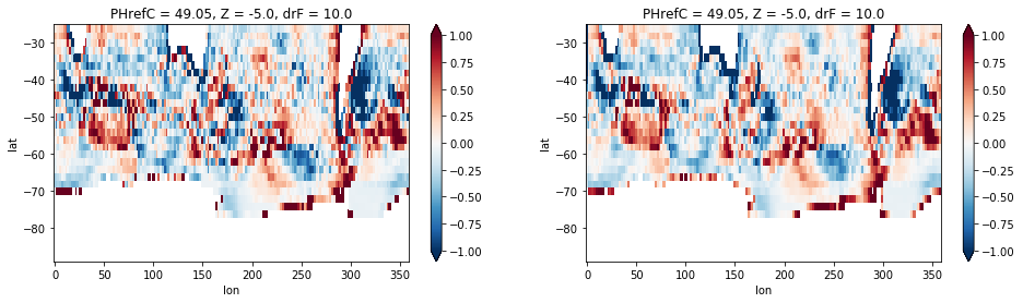
As expected the downsampling (regridding to lower resolution) via interpolation shows more noise. But even in the conservative regridding case there are still many alternating positive and negative anomalies, indicative of the fact that the observations so not resolve features down to the scale of the grid. This is a common issue with observational datasets, which have to use smoothing techniques to aquire a gridded dataset from point measurements.
So lastly we will conservatively regrid both datasets to an even coarser resolution (Method 3.) to alleviate some of this problematic.
To do this we define a coarse global grid using xesmf.util.grid_global and cut it appropriately (remember to leave the bounding coordinates lon_b and lat_b one element longer).
coarse_grid = xe.util.grid_global(5,5).isel(y=slice(0,16), y_b=slice(0,17))
coarse_grid
<xarray.Dataset>
Dimensions:  (x: 72, x_b: 73, y: 16, y_b: 17)
Coordinates:
    lon      (y, x) float64 -177.5 -172.5 -167.5 -162.5 ... 167.5 172.5 177.5
    lat      (y, x) float64 -87.5 -87.5 -87.5 -87.5 ... -12.5 -12.5 -12.5 -12.5
    lon_b    (y_b, x_b) int64 -180 -175 -170 -165 -160 ... 160 165 170 175 180
    lat_b    (y_b, x_b) int64 -90 -90 -90 -90 -90 -90 ... -10 -10 -10 -10 -10
Dimensions without coordinates: x, x_b, y, y_b
Data variables:
    *empty*
Now we define two new regridders and create dataarrays like before. First with the modified model grid and the new coarse grid:
regridder = xe.Regridder(modified_grid_model, coarse_grid, 'conservative') #since this is global we need to pass periodic
regridder.clean_weight_file()
sst_coarse_model = regridder(sst_model.isel(lon=slice(0,-1), lat=slice(0,-1)))
Create weight file: conservative_319x2159_16x72.nc
Remove file conservative_319x2159_16x72.nc
/srv/conda/envs/notebook/lib/python3.7/site-packages/xesmf/smm.py:70: UserWarning: Input array is not C_CONTIGUOUS. Will affect performance.
  warnings.warn("Input array is not C_CONTIGUOUS. "
Then with the modified model grid and the new coarse grid:
regridder = xe.Regridder(modified_grid_obs, coarse_grid, 'conservative') #since this is global we need to pass periodic
regridder.clean_weight_file()
sst_coarse_obs = regridder(sst_obs)
Create weight file: conservative_32x180_16x72.nc
Remove file conservative_32x180_16x72.nc
As a final step we visualize all four comparisons next to each other usign a Stereographic projection of the South Pole:
import cartopy.crs as ccrs

fig, axarr = plt.subplots(ncols=2, nrows=2, subplot_kw={'projection':ccrs.SouthPolarStereo()}, figsize=[15,15])

for ds, ax in zip([sst_model - sst_obs_regridded, sst_model_regridded - sst_obs, sst_model_regridded_cons - sst_obs, sst_coarse_model - sst_coarse_obs],
                  axarr.flat):
    ds.plot.contourf(ax=ax, levels=21, vmax=1, x='lon', y='lat', transform=ccrs.PlateCarree())
    ax.set_extent([-180, 180, -90, -30], ccrs.PlateCarree())
    ax.coastlines()
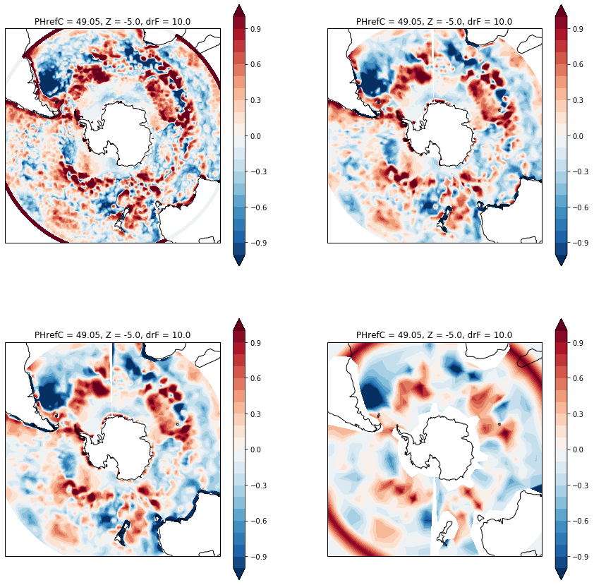
Ultimately which method you use will depend on the particular use case. Before regridding, carefully inspect your datasets and think of what you want to achieve:
Are both datasets of a similar resolution and relatively smooth? Then using linear interpolation should be acceptable and is by far the easiest way to compare the datasets.
Is the goal of the comparison to evaluate differences on larger scales than the grid scale? Then create a coarser grid and interpolate conservatively to gain a larger scale perspective without getting distracted by smaller scale features.