Assignment: Calculate wet bulb temperature for CMIP6 models
Assignment: Calculate wet bulb temperature for CMIP6 models#
Global temperatures are increasing due to the effects of anthropogenic greenhouse gas emissions. This has many potentially disastrous consequences for many people around the world. One of the concerns is that in hot and humid climates, depending on the humidity and increase in temperature could lead to fatal conditions. One way to quantify the combined effect of temperature and humidity for human health is the wet bulb temperature (WBT), which can be approximated as:

“The wet-bulb temperature is the lowest temperature that can be reached under current ambient conditions by the evaporation of water only”. Simply put, if the wet bulb temperature gets too high, the evaporation of sweat can not cool the human body sufficiently.
A sustained wet bulb temperature >35C is likely to be fatal, but lower WBT can also be dangerous depending on other external factors (e.g. solar radiation and insufficient air flow). From Raymond et al. 2020: “for example, regions affected by the deadly 2003 European and 2010 Russian heat waves experienced TW values no greater than 28°C”
This exercise aims to practice working with the CMIP6 cloud archive by computing the wet bulb temperature from available variables and summarizing the results in timeseries plots.
Lets start by importing matplotlib, xarray, numpy, and combined_preprocessing from xmip.preprocessing. Set the default figure size to (12, 6).
Then load the intake-esm collection for CMIP6 data on Google Cloud Storage (you can use xmip, as we did in the lecture, or set this up according to the pangeo instructions). The result should be the same.
The ingredients we need for wet bulb temperature are surface temperature and relative humidity.
Find the relevant variables using the spreadheet from the lecture. You can enter multiple variables in the search query like so:
.search(..., variable_id=['a', 'b'], ...).
Select a subset of the variables, the
'historical'experiment, the native model grid, monthly output, thres models (['NorESM2-MM', 'MPI-ESM1-2-LR', 'CanESM5']are recommended but feel free to explore), and a single member ('r1i1p1f1') for starters. Check out some more models/members later if you are curious!
Then load the data into a dictionary of xarray datasets like we did in the lecture.
Now lets calculate the wet bulb temperature according to the formula above. Write a function that calculates wet bulb temperature from temperature and humidity.
🚨 Watch the units and convert if necessary! You can always check the units by looking at the metadata of a variable (
ds['your_variable'].attrs['units]).
A good test to see if your function is doint the right thing is to calculate the example from the paper: For relative humidity of 50% and temperature of 20C, we expect ~13.7C for the wet bulb temperature.
To get an idea of the extremes globally lets compute the 90th percentile (
xarray.DataArray.quantile()is your friend) of wet bulb temperature at every timesteps and then compute the annual average of that and plot is as a timeseries for each model.
What we are really interested in is to see how these extreme WBT are going to evolve in the future. Lets use your new CMIP6 skills to get some more data! Make another query to get two of the future scenario experiments (
ssp585andssp245- the ‘worst case’ and ‘middle of the road’ scenarios) for the same models and load them into separate dataset_dictionaries.
Plot the same quantity as before (90th percentile in space and annual maximum) for each model and all 3 experiments to see how each model predicts wet bulb temperature extremes until the end of the century. Use color/linestyle/lineweight to separate the experiments.
As a final step, lets look where these extremes occur. Plot a map of an annual average from 2099-2100 for each model and scenario. Make sure to restrict the colormap to + 30 to see where extremes occur

